
C/2021-A1 Comet Leonard
C/2021-A1 Comet Leonard - Click here for full resolution
Comets belong to some of the most unpredictable objects at the night sky. Upon discovery they are still far away from Earth. As their large elliptical orbits bring them closer to the sun they will increase in brightness. But by how much is anybody’s guess. And whether they will even make it to the sun in one piece is not certain. Even if they do end up near Earth as bright objects, they may only be observable at dawn or dusk. Observing and photographing comets is therefore not always easy.
On January 03, 2021, a new comet was discovered by Greg J. Leonard at the Mount Lemmon Observatory, near Tucson, Arizona in the US. Its calculated orbit would bring it closest to the sun on January 03, 2022. This made it a promising comet for observing late November until mid December in the northern hemisphere, and mid December through to end of January in the Southern Hemisphere. As time went by, there were some speculations that this might become a truly spectacular comet, clearly visible with the naked eye. Observed from the Northern hemisphere, it never reached that level of brightness. Still, the comet had reached magnitude 5-6, making it a perfect object for observing with a modest telescope.
Sky Plot (click to enlarge)
5º FoV + scope display (click to enlarge)
Conditions
On December 3, Comet Leonard was in conjunction with globular cluster M3, a pretty unique event. Unfortunately, local clouds prohibited imaging that day. Luckily, on the evening of December 08, the sky cleared, creating an opportunity for imaging before the comet would disappear to the Southern Hemisphere. In the morning of the 9th, the comet rose above the Eastern horizon at around 05:00h. It allowed imaging from the backyard in Groningen, The Netherlands (53.18, 6.54). Moon had set already by the time the images were taken.
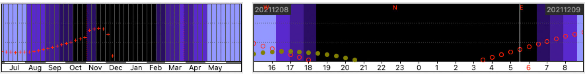
Visibility charts showing 06:00h altitude throughout the year (left) and throughout the session on 09 December, 2021 (right).
Weather was generally good, with temperatures around the freezing point. Humidity was fairly low for this location at 79%. Visibility was reasonably good with SQM values at 19.9 mag/arcsec2. However, as the comet rose further above the horizon, twilight started and the background got brighter quickly. Some of the final photos had to be discarded as the background signal became way too high.

Capturing
The image was captured using the Takahashi FSQ-106 in combination with the QHY268c camera. A one-shot-colour camera is highly preferred, as the fast motion of the comet makes it difficult to combine images from different colour channels. The recently acquired QHY268c, an APS-C sized OSC camera appeared perfect for this occasion. It was difficult to estimate the required field of view, as length of the tail that would be visible under these conditions, as well as the comets motion across the frame were difficult to estimate upfront. The FSQ-106 in combination with APS-C sized camera has a FoV of 2.5º x 1.7º, which turned out to be more than enough to get the comet and all of its visible tail in the frame for almost two hours.
Telescope
Mount
Camera
Filters
Guiding
Accessoires
Software
Takahashi FSQ-106, Sesto Senso 2
10Micron GM1000HPS, Berlebach Planet
QHY268c, cooled to -15 ºC
Astronomik 2” L3 UV/IR cut-off filter
Unguided
MacMini 2018 (MacOS 10.14.6), Pegasus UPBv2, Aurora Flat Field panel
KStars/Ekos 3.5.6, INDI Library 1.9.3, Mountwizzard4 2.1.5, SkySafari 6.8.2, openweathermap.org
The image was captured using a standard UV/IR cut-off filter. The motion of the comet was pretty high. It travelled across the stars at a speed of 17 arcsec/min. With a pixel-scale of 1.46 arcsec/pixel this meant that during an exposure of 60 seconds, the comet had crossed 12 pixels. That is too much to keep the nucleus of the comet nice and sharp as can be seen in the images below. Different exposures were tested, but anything of 30s or longer were too much. For final images exposures were kept to 20s per image. Rather short, but at gain 26 (switch-point to a high-gain modus), a decent amount of the comet’s tail was visible. In total 271 frames were shot that had sufficient contrast with the brightening background of dawn.

Image
A total of 271 frames made it into the final stack of the comet, which equals approximately 1.5h of total exposure. The many frames helped to keep the noise well under control. Overall contrast was good, and a decent dust tail can be seen in the image, despite the less than ideal conditions of imaging against a brightening morning sky.

After a little crop to straighten the edges, the final image has a resolution of 5342 x 3568 pixels, or 19.1 Megapixels. It covers a field of view of 2.17 degrees horizontally. The camera was rotated with north pointing to the right. This made the comet to be diagonally moving across the frame. In reality, the tail pointed pretty much upwards, with the comet moving a bit sideways.
Annotated image showing other deep sky objects, stars brighter than mag. 11 and the image’s orientation.
While a stacked photo provides a detailed look at the comet, it does not show the dynamic nature of the comet wandering through the night sky. The following video shows in 27 seconds the distance travelled in almost 2 hours.
Processing
All frames were calibrated with Bias (100), Dark (50) and Flat (25) frames. Then all frames were debayered and registered. This aligns the stars, but if you Blink the images, the comet will move position between frames. So a second alignment is needed on the comet. To achieve this, there is a special process within PixInsight, called CometAlignment, that makes this process quite easy. First, all registered images (star aligned) were loaded in the tool. Then one image was selected as reference image. This defines the geometry of the final image. Typically an image somewhere halfway the list works well. The first and last image were opened by double clicking on them in the list. Then in each image the location of the nucleus of the comet was selected. The selection is indicated with a green circle.
The Comet Alignment process in PixInsight
Selecting both centers populates the Parameters section in the CometAlignment tool. An output directory was selected and with the Subtract section still empty, the images processed. The images now all had the comet aligned. These images were combined with a regular ImageIntegration, using Linear Fit Clipping as the rejection method (low: 4, high: 1). The resulting image was a starless image.
Back to the CometAlignment process again, and another output directory was selected, as well as another postfix. This time, the image just created with the comet only was selected as the Operand Image. LinearFit disabled gave better results, but this is open for experimentation.
The resulting stars-only images were then combined using ImageIntegration into a star-only image. Finally, the CometOnly image and the StarsOnly image were combined using a simple PixelMath expression.

From here, regular processing took place, including a dynamic crop to crop away some artefacts introduced at the edges during the dual registration process. A combination of DBE and ABE were used for background extraction. Background neutralisation and ColorCalibration were used to get the colours right. Noise was then reduced using the true and tested MMT noise reduction method.
For stretching to the non-linear stage, a lot of attention was on keeping the colours correct. Usually this works better with ArcSinhStretch, and in this case a combination together with Histogram Transformation was used. Once in linear stage, not much had to be done. A bit more contrast using Curves Transformation and some finishing touches in Photoshop created the final image.
Video
For the video, all 271 images had to be processed individually. The calibrated, debayered and registered images were used that were created for the photograph. They were all put in an Image Container. This Image Container was placed on a Process Container with two processes: Dynamic Crop and Automatic Background Extraction. Using the containers allowed a great deal of automation of the processing of all individual images.
Stretching so many images was a bit of a challenge, but eventually the Blink tool was used for it. Blink contains a menu item to make animated GIF’s. So with individual unlinked stretching selected, this process was run, which gave 271 individual stretched PNG-files. In some of them, satellite stripes were visible. They were removed in Photoshop using the content-aware spot healing brush tool. All clean PNG’s were then loaded into Final Cut Pro X to combine them into a 4K video.
Processing workflow (click to enlarge)
This image has been published on Astrobin.