
Comet C/2022 E3 (ZTF) 1/2
Comet C/2022 E3 (ZTF) - Click here for full resolution
Discovered on 02 March 2022, Comet C/2022 E3 (ZTF) was spotted as a very faint 17.3 magnitude smudge in the constellation of Aquilla. The 1.2m telescope at Zwicky Transient Facility (ZTF) is crowned with the comet’s discovery. Based at the Palomar Observatory in California, this facility is designed to detect transient objects that rapidly change in brightness. C/2022 E3 (ZTF) is a long period comet with an estimated orbital period of at least 50,000 years and is expected to reach perihelion on 12 January 2023. E3 will then reach closest approach to the Earth on 01 February 2023. It is unlikely that C/2022 E3 (ZTF) will get as bright as comet Neowise in 2020. However as with all comet brightness predictions, nothing can be ruled out. The most optimistic predictions say that the comet may reach magnitude +5 at a stretch so it is possible that E3 comes within naked eye brightness. At the time of imaging C/2022 E3 was residing in the constellation of Bootes and had reached about magnitude 9.2. The comet is headed towards Draco and Ursa Minor through January 2023 steadily increasing in brightness along the way. Follow the actual position on The Sky live.
Source: CometWatch
Comet: C/2022 E3 (ZTF)
Other Names: n.a.
Object: Comet
Constellation: Bootes
R.A.: 15h 37m 58s
Dec: +46º 03.7’
Closest to Sun: 12 January 2023
Closest to Earth: 01 February 2023
Sky-plots with a FoV of 50º (left) and 5º (right). Click to enlarge
Visibility
Images were taken on the early morning of 18 January 2023 from the backyard in Groningen, The Netherlands (53.18, 6.54). The comet will likely be at its brightest by the end of January. By that time it is very high in the sky and visible throughout most of the night. On 18 January, observing in the evening was very challenging as the comet was very low in the sky. Anywhere from 02:00h visibility was pretty good. However, this was too early to get out of bed for my liking, so I got up at 05:00h and started the session then. Imaging was done until dawn, around 07:00h.
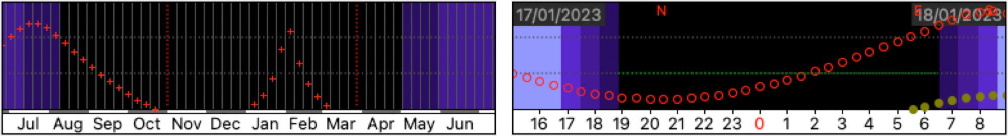
Visibility charts showing 22:00h altitude throughout the year (left) and throughout the session on 18 January, 2023 (right).
Weather
Conditions were pretty good. The moon was absent, the sky was nicely clear and dark and humidity was not too bad.

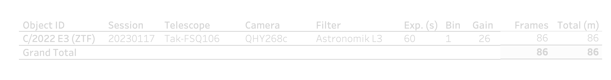
Imaging
It was not completely clear how long the tail of the comet would be. Therefore the FSQ-106 was reduced with the 645 super reducer QE 0.72x. The resulting focal length of that system is 382mm. In combination with the APS-C sized sensor of the QHY268c this gives a Field of View of 3.6º x 2.4º. Imaging a comet with a monochrome camera and colour filters is a bit challenging because of the movement of the comet. So the choice was made for a One Shot Colour camera in combination with a luminance filter, the Astronomik L-3.
Telescope
Mount
Camera
Filters
Guiding
Accessoires
Software
Takahashi FSQ-106, 0.72x 645 Reducer, Sesto Senso 2
10Micron GM1000HPS, EuroEMC S130 pier
QHY268C, cooled to -15 ºC
2” mounted Astronomik L-3, Baader filter drawer
Unguided
Fitlet2, Linux Mint 20.04, Pegasus Ultimate Powerbox v2, Aurora Flatfield, MBox
KStars/Ekos 3.6.2, INDI Library 1.9.9, Mountwizzard4 2.2.9, PixInsight 1.8.9-1

Geometry
Resolution
Focal length
Pixel size
Resolution
Field of View
Rotation
Image center
5391 x 3589 px (19.3 MP)
382 mm @ f/3.6
3.76 µm
2.02 arcsec/px
3º 31’ x 2º 20’
-17.1 degrees
RA: 15º 37’ 58.218”
Dec: +46º 03’ 44.46”
Processing
All frames were calibrated with Dark (50) and Flat (25) frames and registered using the WeightedBatchPreprocessing (WBPP) script. WBPP has an option to split the R,G and B channels from an OSC image during the debayering process. In that way, each colour channel is registered independently. This can help keeping the colour of the stars more uniform. Especially at the edges of the frame stars can show a bit of a ‘rainbow’ effect, which is somewhat suppressed by this technique. Downside is of course that there is three times so many frames to deal with in further processing.
Processing of a comet is challenging in that over the course of the session, the comet will move quite considerably across the star field. This means that aligning the images on the stars will smear out the comet, and aligning the images on the comet will smear out the stars. So most comet processing techniques do both and have solutions to separate the two first and bring them back together again later. PixInsight has a tool that does exactly this, which is called CometAlignment. This technique was applied when processing comet Leonard. But nowadays there is StarXTerminator, which can run in batch-mode. So one can make a set of comet-only images by simply running the StarXTerminator process on them. Only one drawback, this takes a long time. On my system, each image takes just under two minutes. So extracting 258 images took approximately 8 hours.
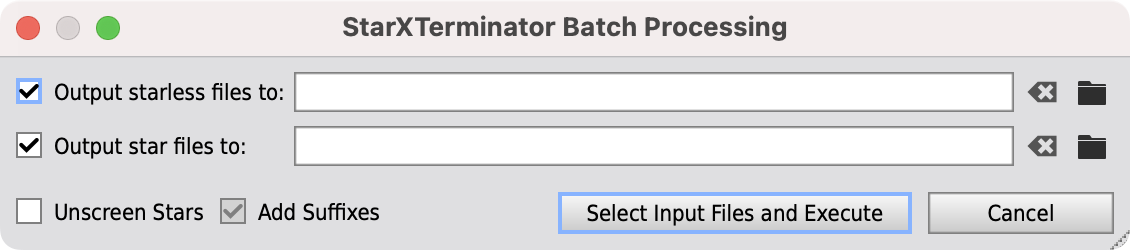
StarXterminator now can run batches of images, making it very easy to create comet-only images. It is quite calculation intensive though, so be prepared for a long wait for the computer to be finished.
Stars
To get to a Stars-only image, the first part of the processing uses ImageIntegration to stack all registered files. The comet then becomes a bit of a smear, but that is no problem. Processing involves the regular sequence of DynamicBackgroundExtraction and SpectroPhotometricColorCalibration. When running SPCC, the white balance adjustment values for each of the red, green and blue channel were written down for later use during comet processing. Next step was BlurXTerminator (BXT). The 0.72x reducer on the FSQ-106 is not completely without its flaws, and stars in the far corners can show some aberrations. BXT helps to correct that a bit, and reduces the star sizes in the process. Running StarXTerminator (SXT) now creates the Stars-only image. SXT did overall a good job, but some remainders of the comet were still in there. A simple CloneStamp operation could easily deal with that. Also at this stage, the image was cropped to eliminate some of left-over edges from the stacking process. The image was stretched using a few runs of HistogramTransformation and colours of the stars were intensified using ColorSaturation.
Comet
Processing the comet was quite a bit more work. First the starless images needed to be aligned on the comet. This process is fairly easy to do using the CometAlignment process in PixInsight. For each channel the frames were combined with ImageIntegration and the resulting red, green and blue stack were then combined to create an RGB image of the Comet-only. After running DBE, it became clear that SXT is not taking out all of the star-signals. Very faint star-trails could still be seen in the background of the Comet-only image. This is very common, as the same happens with the traditional method as well. One could opt to just leave them in and keep them as unobtrusive as possible during stretching. But I chose to clean up at least the biggest trails using the CloneStamp tool. The result was reasonably good, although directly around the comet one needs to be extremely careful not to eliminate anything from the comet structure or its tail.
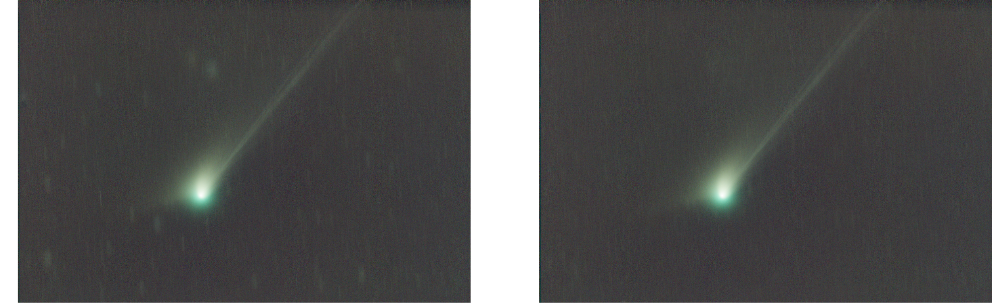
Even when using StarXTerminator to isolate the comet, some faint star trails remain visible, just like often in the traditional method. The starless phase is the perfect timing to eliminate those trails using the CloneStamp tool.
Next up is getting the colours right. How do we know what the real colour of the comet is? At this stage it is impossible for regular colour calibration techniques to come up with the right answer. But we can use the information from the Stars-only image. When SPCC was run on the Stars image, the tool showed the relative adjustments to the red, green and blue channels to get the white balance right. That information was written down. Now this information can be manually entered in the ColorCalibration tool to calibrate the comet’s colour.

The red, green and blue relative adjustment values that SPCC generated for the stars image can be applied to the comet-only image using the manual white balance settings in the ColorCalibration tool.
The same crop from the Stars-only image was now applied to the Comet-only image and a mild noise reduction was applied. For stretching both the GeneralisedHyperbolicStretch and regular HistogramTransformation were tried. While the former was better able to isolate the bright comet’s nucleus, the overall result from the latter was preferred. To still retrieve a bit more detail from the comet’s nucleus, CurvesTransformation was used to lower the highlights a bit. To further clean up the background, some desaturation of the color and removal of green using SCNR was applied while a mask was protecting the comet and its tail.
Final image
To get to the final image, both the Stars-only and Comet-only image were combined in PixelMath. For faint nebulosity images, just adding the two together is usually sufficient. But in this case, there were still some comet left-overs in the Stars-only image that required the slightly more sophisticated technique. A process called screening was used. This blends layers more based on their luminosity, rather than just adding the numbers together. The formula in PixelMath for this is:
combine(CometOnly, StarsOnly, op_screen())
The last steps were just some cosmetic corrections, including a slight increase of brightness of the tail of the comet and an overall further reduction of noise using NoiseXTerminator. In each of the noise reduction steps typically a low value is used to not ‘over-cook’ the effect. But this does mean that at the end of the process there is often some room to do a final cleanup of noise using another run of it.
Processing workflow (click to enlarge)
Animation
As mentioned before, the comet moves across the backdrop of stars at a fairly decent pace. This is clearly visible in a series of images taken over a 1-2h timespan apart. In order to demonstrate this dynamic behaviour, this animation was made.
Basis for this animation were the frames from the green channel. These had the highest image signals. Using the Blink tool, the images were exported as PNG’s with individual stretching applied. These PNG’s were loaded into Photoshop using ‘File > Scripts > Load files in stack’. Since the images were already registered in PixInsight, Photoshop did not have to align them again. Instead they were all loaded as individual layers in one document. Many frames had satellite trails on them. The spot healing brush tool with content-aware setting works perfect to eliminate them. Click the starting point of the trail, hold shift and click the end-point of the trail. A perfectly straight healing brush now takes away the satellite trail. Doing this on 86 images is quite a bit of work, but well worth it. Now turn on the timeline in Photoshop. If it is not visible yet, select it under ‘Window > Timeline’. In the little hamburger menu of the Timeline, the option ‘select all frames’ puts all layers directly on the timeline, which is essentially the animation. An extra layer was added with a title on it. The animation was exported using ‘File > Export > Save for Web (Legacy)’, and using the ‘GIF128 dithered’ preset and 256 colours selected exported. The size was resized to 1000 x 668 pixels, more than large enough for an animation typically viewed on a computer screen.
An animation of the comet moving across the sky. The total animation represents 1h 49m of actual time in the early morning of 18 January 2023
This image has been published on Astrobin.