
Caldwell 34
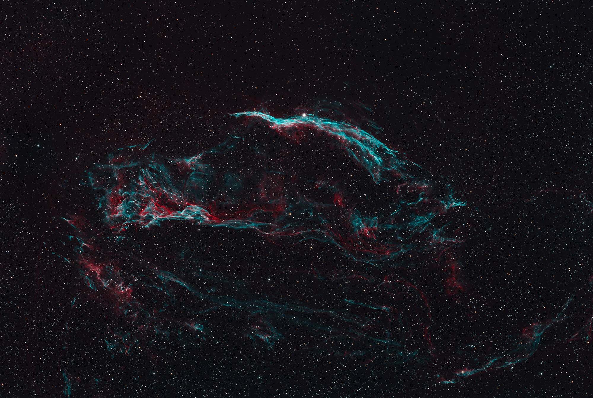
Caldwell 34 - Veil Nebula - Click here for full resolution
Caldwell 34, also known as NGC 6960 or the Veil Nebula, (R.A.: 20h 46m 34.92s, Dec: +30º 47’ 40.9”) is a supernova remnant in the constellation Cygnus at a distance of 2,400 lightyear from Earth. The full remnant consist of the Western (photographed here) and the Eastern Veil Nebula. About 10,000 to 20,000 years ago, this nebula was created when a large star, approximately 20 times the size of the Sun, exploded. Parts of the nebulous area have received their own identifiers. The brightest part, visible at the top in this image, is also known as NGC6960 or the witches broom. On the left in this image is a region known as Pickering’s triangle. The Eastern Veil Nebula, not captured here, would be located below.
Sky Plot (click to enlarge)
5º FoV + scope display (click to enlarge)
Conditions
Images were taken on September 07 and 08, 2021, from the backyard in Groningen, The Netherlands (53.18, 6.54). Moon was absent during both nights. The object was high over the southern horizon, with altitudes between 40 and 65 degrees. After around 3:30h a tree in the garden was blocking the view on the target, so the overall imaging time per night was somewhat reduced.
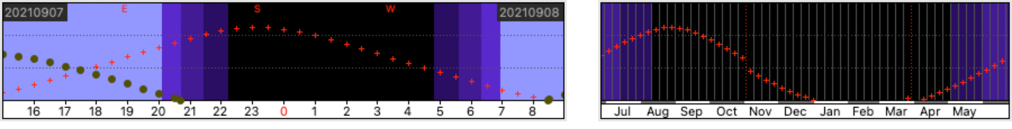
Visibility charts showing altitude at 22:00h throughout the year (right) and on September 07, 2021 (left).
Weather was generally good, with moderate temperatures around 15 degrees Celsius and somewhat high humidity. Visibility was reasonably good with SQM values just touching 20 mag/arcsec2, quite normal for this location.

Capturing
The image was the first object captured using a new mount, the Rainbow Astro RST-135E. This mount has recently been added to the observatory. It combines three objectives: creating the basis for a second rig to maximise use of clear nights, providing a more mobile solution to capture at darker locations and/or less obstructions and being a tracker for more night-scape style astrophotography (Milky Way, meteors, comets, etc).
The RST-135E is unique in that its motors are harmonic drives. This technology is used in robotics. It combines high torque and high precision in a very small form factor. As a telescope mount, this means a small and highly portable mount (3.4kg), that can carry a lot of weight (13.5kg) without the need for counterweights or balancing. A blog describing details of this mount and experiences on how to use it, is in the planning.
The RST-135E mount has no problem carrying the full load of the FSQ-106, ASI6200 plus filterwheel and some accessories without using a counterweight
The first DSO target to be photographed with this mount was the Veil Nebula, using the FSQ-106 with ASI6200 setup. This telescope is right in the sweet-spot of the type of scopes this mount can handle. There were positive reports on using this mount unguided. In reality this was a lot more difficult than expected. It took some trial and error. For unguided to work well, a very good polar alignment should be combined with a good 5-point star alignment model in-mount. But even then, some wobbly stars could be seen on a fairly regular basis. This limited the exposure times to 120s.
Based on the experiences on this image, the setup will be modified to allow for guided imaging. Unfortunately that adds some complexity. On the other hand aligning the mount will be less critical, so overall it can still be an easy to setup system. Unguided use is possible, but probably with a lighter setup in the 200-300mm focal length range. A Redcat type of setup could work well unguided.
Technical Details
Telescope
Mount
Camera
Filters
Accessoires
Software
Takahashi FSQ-106, Sesto Senso 2
Rainbow Astro RST-135E, Berlebach Planet Small
ZWO ASI6200MM Pro, cooled to -15 ºC
Chroma 2” Ha (3nm), OIII (3nm), LRGB unmounted, ZWO EFW 7-position
Fitlet2 (Linux Mint 20.04), Pegasus Ultimate Powerbox v2
KStars/Ekos 3.5.4, INDI Library 1.9.1, openweathermap.org
Frames
The Veil Nebula photographs very well in narrow-band, with strong signal in both H-alpha and OIII. A total of 106 frames of H-alpha and 97 frames of OIII were captured. The disadvantage of narrow-band imaging is that proper star-colour is usually difficult to maintain. To make sure stars don’t just come out white, a small set of RGB exposures does wonders. In this case 20 frames of 30s were recorded for each filter, using 2x2 binning. The higher sensitivity of the binning offsets the short 30s exposure times.

Image
The limitation of the exposure times to 120s meant that the individual frames were somewhat underexposed. 300s Exposures would have been able to collect a lot more detail and brightness in the nebula. Also, the small wobble that was visible in certain frames means that the finest sharpness and detail is a bit lost compared to what is possible. Also, with all the focus being on trying to get unguided imaging working, focus was off at some points. Temperature dropped quickly over the night and the standard once per hour focusing may not have been enough. Despite these drawbacks, the image came out fairly well with a lot of structure and colour nuances.
The RGB colour was exceptionally short, but with the binning enough signal was obtained and it resulted in nice star colours.

After a little crop to straighten the edges, the final image has a resolution of 9390 x 6306 pixels, or 59.2 Megapixels. It covers a field of view of 3.8 degrees horizontally. There are many ways to frame the veil nebula, either zooming in to specific areas, or zooming all the way out to capture both Western and Eastern Veil. This image is somewhere in between.
Annotated image showing other deep sky objects, stars brighter than mag. 9 and the image’s orientation.
Processing
All frames were calibrated with Bias (100), Dark (50) and Flat (25) frames and registered using the WeighedBatchPreprocessing script. During registration, 12 OIII frames were unable to register and dropped out. Therefore the final image, in contrast to what is mentioned in the tables above, only contains 85 frames of OIII. The reason for lack of registration is still unknown, but it was discovered all the way at the end of the process. It was considered not to be worthwhile trying to fix the registration error and repeat the full image processing. But it does stress the importance of checking logs when using automated scripts.
Before image integration, the new NormalizeScaleGradient (NSG) script in PixInsight was applied. This script tries to harmonise the gradient between images to a reference image. Any remaining gradient is then more or less equal between images and easier to remove using DynamicBackgroundExtraction. Also the script applies a weight to each frame for integration that more accurately describes the actual quality of that frame. The usual noise-based weighting can incorrectly assign a high weight to images that got bright because of for example clouds in the frame. The result should be a more contrasty image. For anyone interested, Adam Block has published three YouTube videos where he explains the tool, how to use it and what to expect from it.
In real use, NSG did indeed give a slightly higher contrast to the final image. There were no strong gradients visible in the frames, so the effect on gradients was difficult to assess. It seemed strange that a handful of frames which were partly blocked by trees, had significantly higher weights than the rest. Anyway, it seemed that on balance this script is worthwhile using. It is very processor-intensive, but a helpful nuance is that the script gives an overall estimated time to finish. NSG will likely be embedded in the default workflow. That workflow will then be as follows. Calibration and registration using the WeighedBatchPreprocessing script, apply NSG for each colour channel, followed by image-integration. The script actually populates the ImageIntegration process with the right parameters when finished.
The rest of the processing followed a very similar pattern to earlier images. A DynamicBackgroundExtraction on the integrated H-alpha and OIII images, followed by cropping away the black edges. Noise reduction using the MMT-based method. and then ChannelCombination to assign H-alpha to Red and OIII to Green and Blue. A manual stretch brought the images into the non-linear stage. On the left side of the image there was a reflection of something, causing a bit of a bright blob in the background. Possibly reflections of a bright star, or some kind of light leakage in the system. It was removed by applying a small round of HistogramTransformation using an inverse mask on the blob. This technique worked actually remarkably well. Using the GAME script to create elliptical masks shows very helpful. In the overall image the red was a little bit enhanced and the stars were reduced a bit using MorphologicalTransformation.
The star colour was obtained from the RGB frames. They were collected in 2x2 binmode, so at much lower resolution. However, during registration, these images were automatically up-sized to match the other images. Frames were simply stacked and cropped the same as the other frames. No background corrections were applied, the focus was completely on the colour of the stars. Colour was calibrated using PhotometricColorCalibration, which actually is very easy to use, and often gives very good results. For the first stretching pass, the tool ArcsinhStretch was applied. This is a stretching tool known for maintaining a lot of colour also in brighter areas such as bright stars. For full stretching, an additional run of HistogramTransformation was applied. The contrast was a bit enhanced, and the overall image was smoothened using convolution, which sort of acts as a noise reduction. A very important step is to make sure that the brightness of the stars in the RGB and HOO images are the same. This was done by extracting the luminance channel from the HOO image, and apply it to the RGB image using LRGBCombination. Now the star colour can be added to the HOO image using simple Pixelmath, as long as there is a good star mask in place. Final finishing touch was done by enhancing contrast (CurvesTransformation) and some dodging and burning in Photoshop.
Processing workflow (click to enlarge)
This image has been published on Astrobin.